September 15, 2021
Statistics for Data Science

DURATION
15mincategories
Tags
share
Generally, statistics is a graphical and mathematical representation of information. Data science is all about performing on data. On the premise of that data we make decisions, with the help of some mathematical conditions which are called models, within the term of machine learning.
There are two varieties of statistics:
1. Descriptive statistics
2. Inferential statistics
1. Descriptive Statistics
In descriptive statistics we see analysis, summary and organization of data within numbers, graphs, bar plots, histograms, charts, etc.
2. Inferential Statistics
Inferential statistics is predicated on conclusion. We apply any mathematical and logical operations on data, then we conclude our result within forms of accuracy, confidence intervals, and hypothesis testing.
We divide statistics into three parts:
Basis statistics
Intermediate statistics
Advanced statistics
In this article we are going to learn about basic statistics. Below are the subjects we’ll explore with the assistance of theory and code.
1. Introduction to basic terms
2. Variables
3. Random variables
4. Population, sample, population mean, sample mean
5. Population distribution, sampling
6. Mean, median, mode
7. Range
8. Measure of dispersion
9. Variance
10. Standard deviation
11. Gaussian distribution
Statistics allow us to see information because statistics relies on data. Data is a collection of information in any form (numerical, text, graph, images, etc.).
Data may be represented any way. For example, census or graphical data, also within the variety of images, audio and video.
Population and Sample
Population is a complete dataset on which we want to do some analysis. A sample is some random small data taken from a population, such that it contains at least one member of all the dataset. This selection should be done in an unbiased way.
Population Mean and Sample Mean
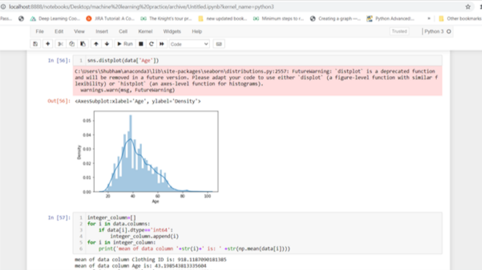
Population mean is the average of a complete dataset. On the other hand, sample mean is a mean taken on randomly selected sample data from the population data, and its mean denoted by µ1. The difference between population mean and sample mean is called marginal error, or sampling error. If all sample data is taken in an unbiased way, then this error will be 0.
1 2 3 4 5 6integer_column = [] for i in data.columns: if data[i].dtype == 'int64': integer_column.append(i) for i in integer_column: print('mean of data column ' + str(i) + ' is: ' + str(np.mean(data[i])))
Variables
Variables are those values that are not given. For example, if we have to find the average weight of all the men in a given data set.
This notation tries to equalize the future computational value to current symbols, like the age of a person as Y=f(x)-f(x+1). Here, x and y are the variables.
Random Variables:
A random variable is usually written as a capital letter, like ‘X’, and is a type of variable whose possible numerical value is the outcome of random experiments. For example, there are around seven billion people in the world and you want to find the total number of people whose age is over fifty years, then this age is a random variable.
There are two type of random variables:
Discrete random variables
Continuous random variable
Discrete Random Variables
In discrete random variables the value of the random variable is finite and within a particular range, like the number of a certain gender in a population.
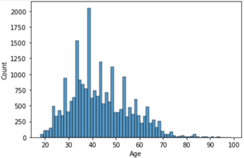
For the probability distribution of discrete random variables we typically use a histogram plot.

Continuous Random Variables
Continuous random variables have an infinite range of values; these are generally part of the experiments, like speed, velocity, distance, weight, etc.
They generally contain some interval-based value. For example, when we plot on a number line we get some interval based like -1<x<1, here (-1,-1) is range, x is the continuous variable.
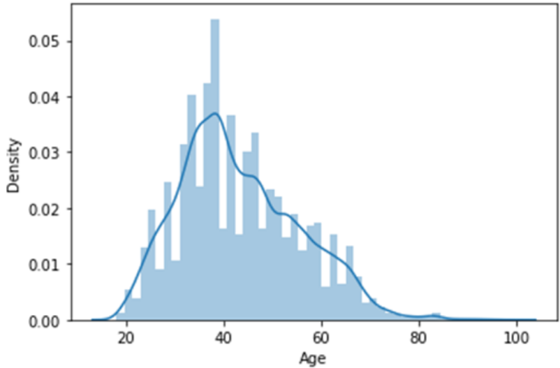
To plot the probability for a continuous random variable we use a normal/gaussian plot.
Normal (Gaussian) Distribution
A normal distribution is a mean-centred, bell shaped,symmetric curve in which mean is µ=0 and standard deviation σ is 1. This curve is basically used for abnormalities or outliers in our dataset, like the percentage of a dataset which are close to mean and standard deviation.
If the dataset follows the normal distribution, then 68% of the data will be in the first range of z-score, 95% percent of data will be in the second range of standard deviation, and 99.7% of data will be in the third range of standard deviation.
The equation of a normal distribution curve is
Y=
(σ± µ) 68% dataset (-1,-1)
(σ± 2µ) 95% dataset (-2,2)
(σ± 3µ) 99.7 % dataset (-3,3)

